3 Dataset creation
3.1 Definition and content
As explained in Section 1.2.1, the main requirements of the dataset that I wanted to create were to contain at the same time LiDAR data, RGB data and CIR data, with simple bounding box annotations for all trees, including trees that are partially or completely covered by other trees (see Section 2.2).
Then, to make the most out of the point cloud resolution and the RGB images resolution, I decided to use a CHM resolution of 8 cm, which is also the resolution of the RGB images. However, the resolution of CIR images is 25 cm, which made it less optimal, but still usable.
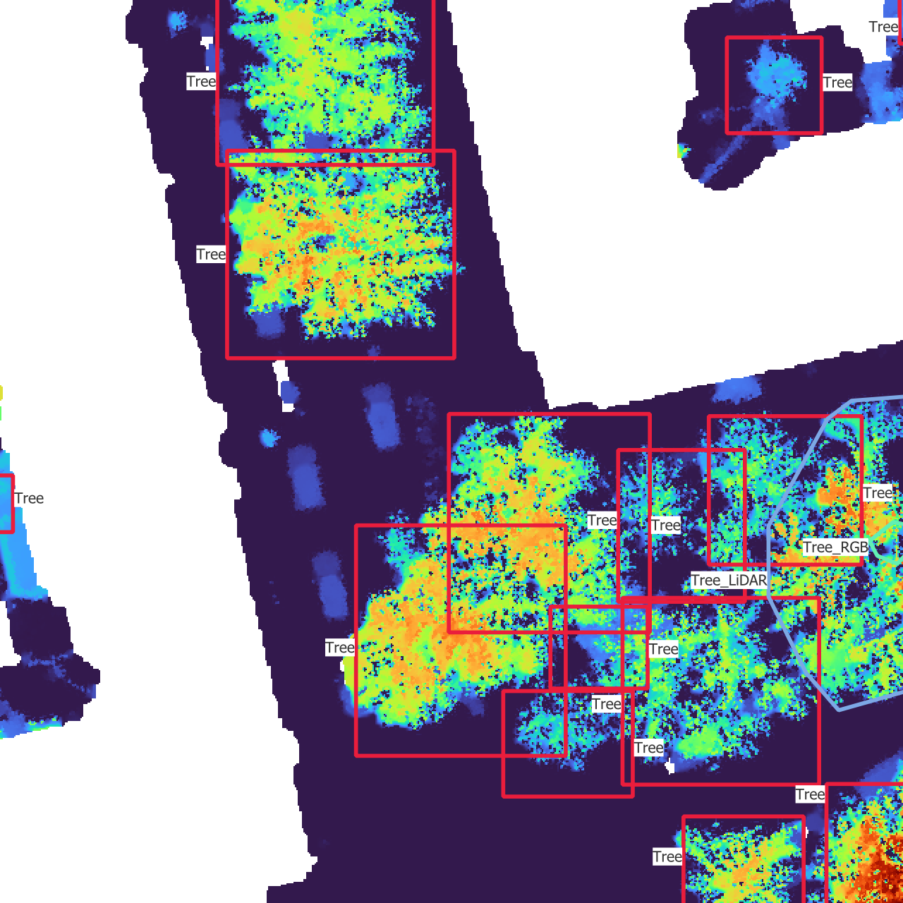
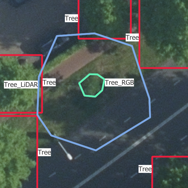
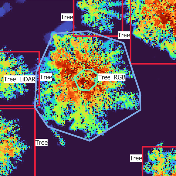
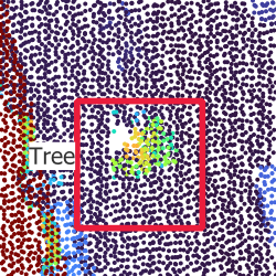
To be able to get results even with a small dataset, I decided to focus on one specific area, to limit the diversity of trees and environments to something that should still be learnt with a small dataset. Therefore, the whole dataset is currently inside of a 1 km × 1 km square around the Geodan office in Amsterdam. It contains 2726 annotated trees spread over 241 images of size 640 px × 640 px i.e. 51.2 m × 51.2 m. All tree annotations have at least a bounding box, and some of them have a more accurate polygon representing the shape of the crown. There are four classes, which I will detail in the next section Section 3.3, and each tree belongs to one class.
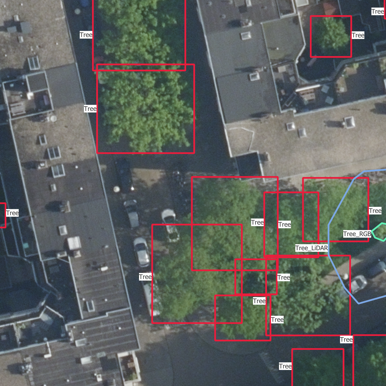
On Figure 3.1, you can see what the dataset finally looks like, with all data sources and bounding boxes.
3.2 Data annotation setup
Annotating all these trees took me about 100 hours, with a very high variation of the time spent per tree depending on the complexity of the area. To make the most out of the different data types and fully use them, I mainly used four data sources and tools.
The most important tool I used is QGIS (QGIS Development Team, n.d.). QGIS allowed me to visualize all types of data on the same map: images, point clouds, CHM rasters, boxes and polygons. I therefore used it to annotate the trees, switching between RGB images and LiDAR point clouds to detect individual trees. One very useful feature of QGIS is the possibility to filter the point cloud based on some properties of the points. I mainly used it to filter out all the points that were classified as buildings and to adapt the height interval to make the most out of the color gradient and get rid of the ground or the large trees. This way of removing part of the point cloud using height thresholds is also related to the idea of having multiple CHM layers fed into the model using height intervals of the point cloud.
However, QGIS is mostly limited to 2D views from the top, which doesn’t benefit from the 3D aspect of the point cloud. To visualize the point cloud, I used the official viewer provided with the AHN4, called AHN-puntenwolkenviewer, which means AHN point cloud viewer (Actueel Hoogtebestand Nederland, n.d.). This viewer allows to navigate through the point cloud, see it from different angles and color the points according to different attributes. I found the intensity (intensiteit) to be a convenient way to display the point cloud, as it sometimes allow to differentiate between leaves and branches, and it breaks the homogeneity of using the height as color attribute. This viewer enabled me to make sense out of the 2D view of the point cloud I had in QGIS.
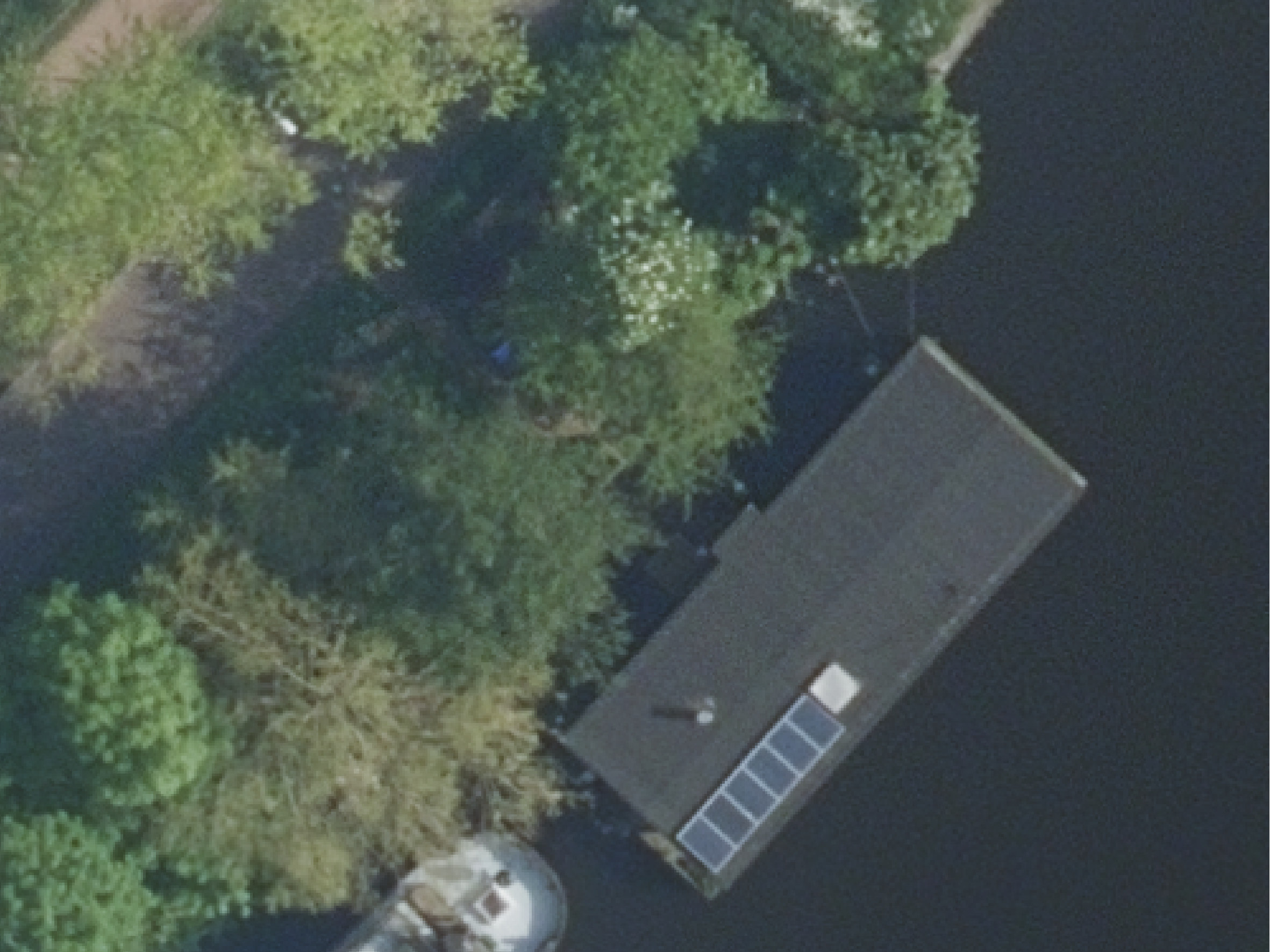
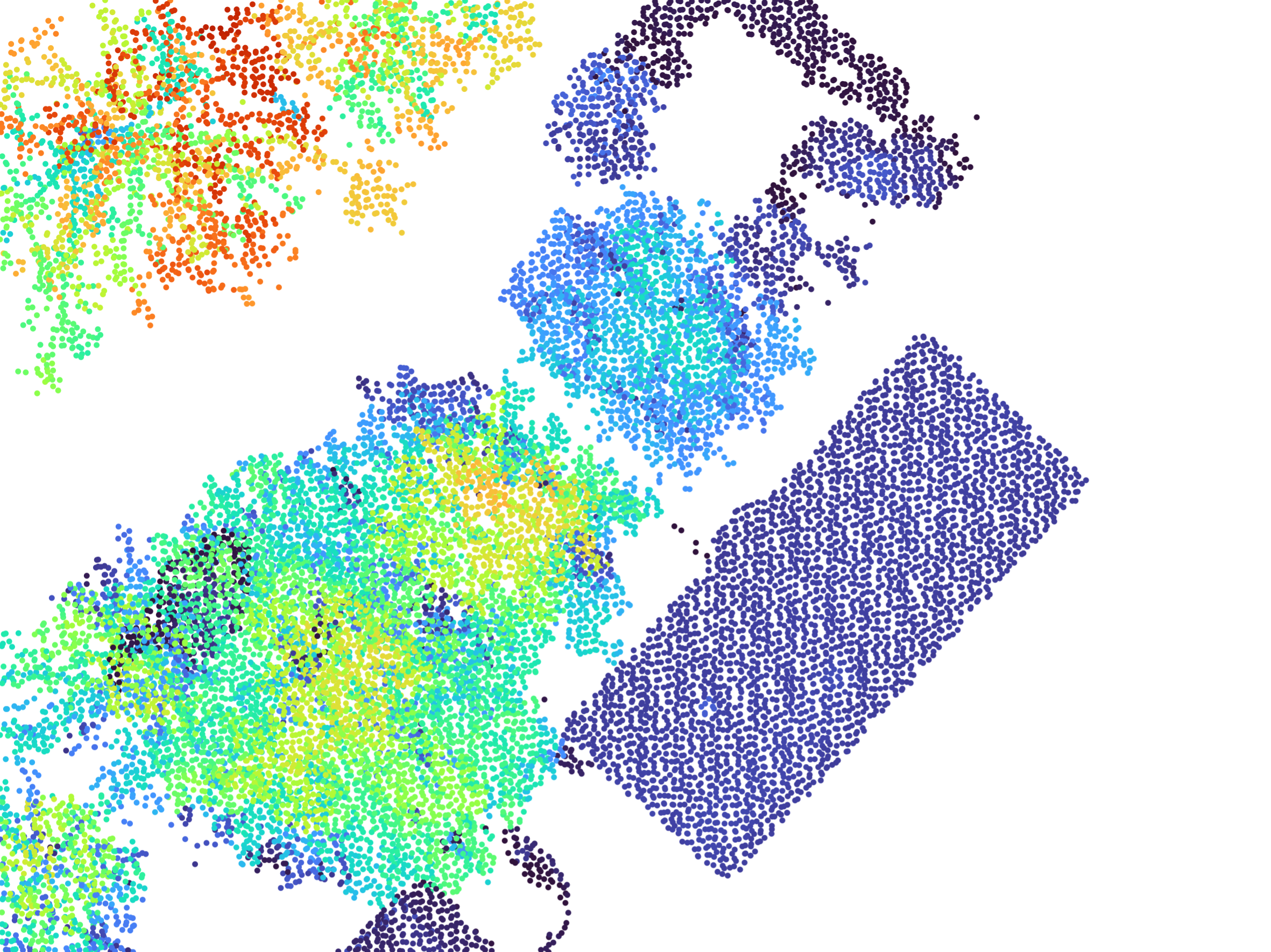
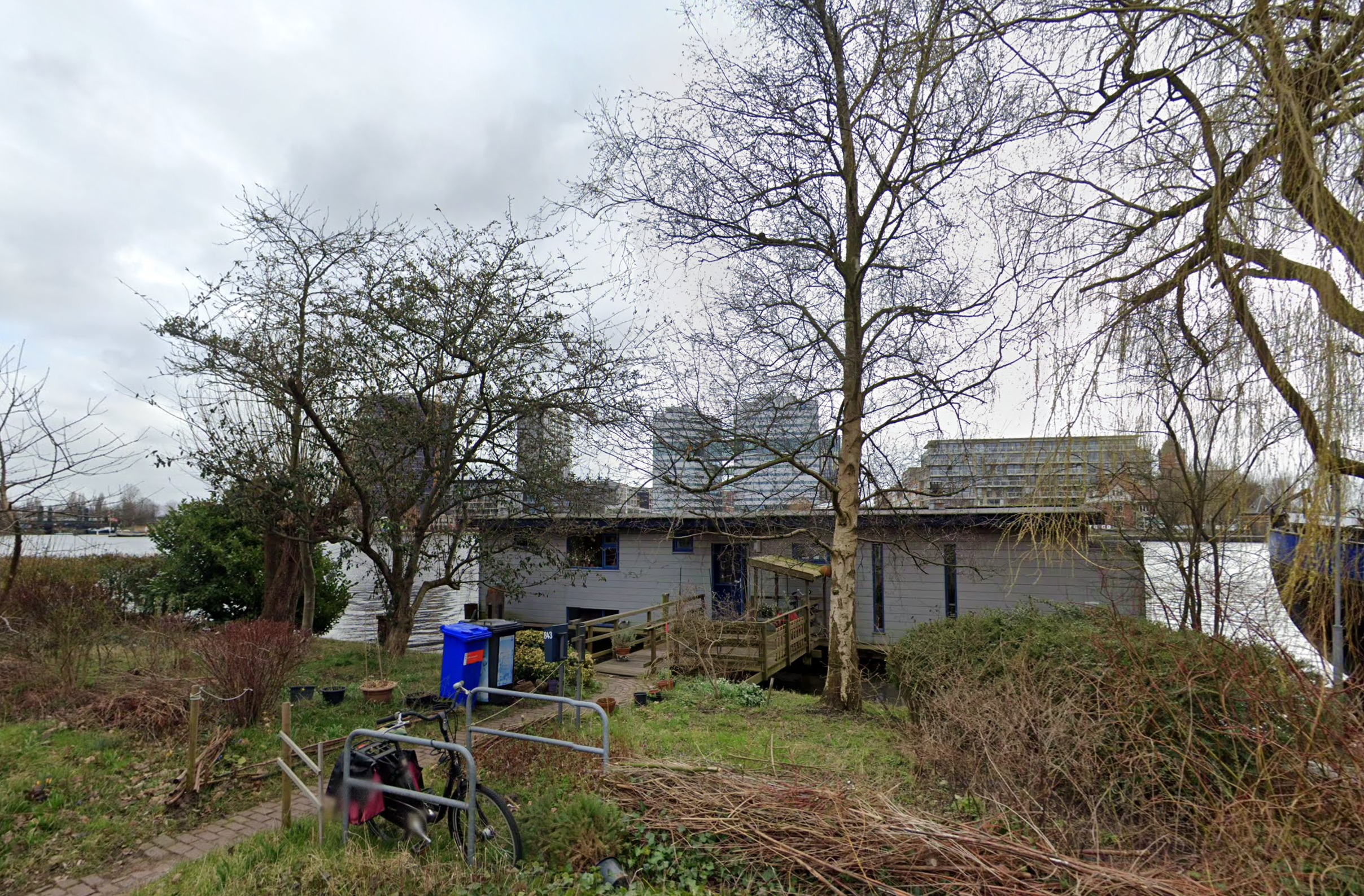
Finally, I also used Google Street View (Google 2024) to have visual information about the trees. This was mainly useful for the most difficult parts of the dataset, but it was only available for trees that were not too far from a street. Google Street View images helped me in dense areas with thin trees, where the point cloud doesn’t capture very well the structure of the trees and trees are mostly indistinguishable from above. Having the possibility to switch between different dates also enabled me to see the evolutions and have more chances to find a clear picture.
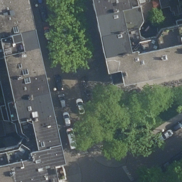
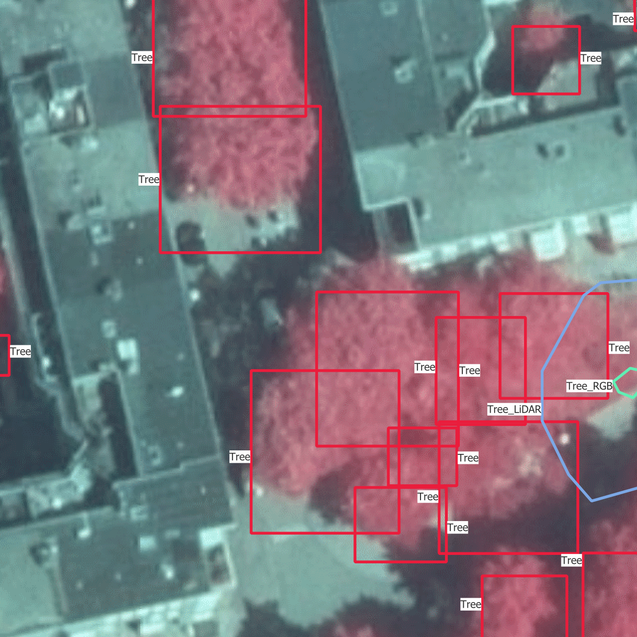
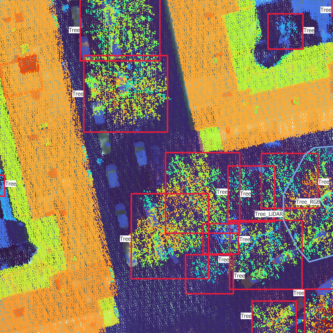
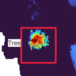
In Figure 3.2, you can see what each data source looks like.

3.3 Challenges and solutions
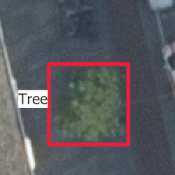
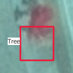
The creation of this dataset raised a number of challenges. The first one was the interval of time between the acquisition of the different types of data. While the point cloud data dated from 2020, the RGB images were acquired in 2023. It would have been possible to use images from 2021 or 2022 with the same resolution, but the quality of the 2023 images was much better, in the sense that trees were much more distinguishable. Consequently, there were a certain amount of changes regarding trees between these two periods of acquisition. Some large trees were cut, while small trees were planted, sometimes even at the position of old trees that were previously cut in the same time frame. For this reason, a non negligible number of trees were either present only in the point cloud, or only in the images. An example of such a situation can be found in Figure 3.3. To try to handle this situation, I created two new class labels corresponding to these situation. This amounted up to 4 class labels:
- “Tree”: trees which are visible in the point cloud and the images
- “Tree_LiDAR”: trees which are visible in the point cloud only but would be visible in the images if they had been there during the acquisition
- “Tree_RGB”: trees which are visible in the images only but would be visible in the point cloud if they had been there during the acquisition
- “Tree_covered”: trees that are visible in the point cloud only because they are covered by other trees.
The next challenge was the misalignment of images and point cloud. This misalignment comes from the images not being perfectly orthogonal. Point clouds don’t have this problem, because the data is acquired and represented in 3D, but objects in images have to be projected to a 2D plane after being acquired with an angle that is not perfectly orthogonal to the plane. Despite the post-processing that was surely performed on the images, they are therefore not perfect, and there is a shift between the positions of each object in the point cloud and in the images. This shift cannot really be solved, because it depends on the position of the object relative to the sensor. Because of this misalignment, a choice had to be made as to where tree annotations should be placed, using either the point clouds or the RGB images. I chose to the RGB images as it is simpler to visualize and annotate, but there was not really a perfect choice.
On Figure 3.4, you can see two of the issues. First, you can see that a bounding box that is well-centered around the tree in the RGB image is completely off on the CIR image, and also not really centered on the CHM raster. Then, you can see that the bounding box is much smaller on the CHM, mainly for two reasons: the tree grew between the acquisition of the LiDAR point cloud and the RGB image and small branches on the outside of the tree are hard to capture for LiDAR beams.
Finally, the last challenge comes from the definition of what is considered as a tree and what is not. There are two main sub-problems. The first one comes from the threshold to set between bushes and trees. Large bushes can be much larger than small trees, and sometimes have a similar shape. Therefore, it is hard to keep coherent rules when annotating them. The second sub-problem comes from multi-stemmed and close trees. It can be very difficult to see, even with the point cloud, if a there is only one tree with two or more trunks dividing at the bottom, or multiple trees which are simply close to one another. This challenge is also mentioned in another paper (Weinstein et al. 2019). In the end, it was just an unsolvable problem for which the most important was to remain consistent over the whole dataset.
3.4 Augmentation methods
Dataset augmentation methods are in the middle between dataset creation and deep learning model training, because they are a way to enhance the dataset but depend on the objective for which the model is trained. Their importance is inversely proportional with the size of the dataset, which made them very important for my small dataset of annotated trees.
As it was already explained in Section 1.2.4, I used Albumentations (Buslaev et al. 2020) to apply two types of augmentations: pixel-level and spatial-level.
Spatial-level augmentations had to be in the exact same way to the whole dataset, to maintain the spatial coherence between RGB images, CIR images and the CHM layers. I used three different spatial transformations, applied with random parameters. The first one chooses one of the eight possible images when flipping and rotating by angles that are multiples of 90°. The second one adds a perspective effect to the images. The third one adds a small distortion to the image.
On the contrary, pixel-level augmentations must be applied differently to RGB images and CHM layers because they represent different kinds of data, and the values of the pixels do not have the same meaning. In practice, a lot of transformations were conceived to reproduce camera effects on RGB images or to shift the color spectrum. Among others, I used random modifications of the brightness, the gamma value and added noise and a blurring effect randomly to RGB images. For both types of data, a channel dropout is also randomly applied, leaving a random number of channels and removing the others. A better way to augment the CHM data would have been to apply random displacements and deletions of points in the point cloud, before computing the CHM layers. However, these operations are too costly to be integrated in the training pipeline without consequently increasing the training time, so this idea was discarded.
On Figure 3.5, you can see an RGB image and 15 random augmentations of this image, generated with the transformations and the probabilities used during training. The most visible change happens when one or two color channels are dropped, which completely changes the color of the image.But other effects are also visible such as luminosity changes in images n°4 and 14, perspective changes in n°5, 8 and 13, blurring in n°1 and 14, and distortions in n°10 and 12. All these effects and some other less identifiable augmentations (like noise), are randomly combined to produce many different images, with bounding boxes being modified accordingly.