5 Results
In this section are the results of the experiments performed with the model and the dataset presented before.
5.1 Training parameters
The first experiment was a simple test over the different parameters regarding the training loop. There were two goals to this experiment. The first one was to find the best training parameters for the next experiments. The second one was to see if randomly dropping one of the inputs of the model (either RGB/CIR or CHM) could help the model by pushing it to learn to make the best out of the two types of data.
The different parameters that are tested here are:
- “Learn. rate”: the initial learning rate.
- “Prob. drop”: the probability to drop either RGB/CIR or CHM. The probability is the same for the two types, which means that if the displayed value is 0.1, then all data will be used 80% of the time, while only RGB/CIR and only CHM both happen 10% of the time.
- “Accum. count”: the accumulation count, which means the amount of training data to process and compute the loss on before performing gradient back-propagation.
As you can see on Figure 5.1, sortedAP reaches at best values just above 0.3. Since the dataset is small, the training process overfits quickly, and the model doesn’t have enough training steps to have confidence scores which reach very high values. As a consequence, it is difficult to know beforehand which confidence threshold to choose. Therefore, the sortedAP metric is computed over several different confidence thresholds, and the one that gives the best value of sortedAP is kept. This is why the name of the column is “Best sortedAP”, as the highest sortedAP value over several confidence thresholds is displayed.
This experiment shows that a learning rate of 0.01 seems to make the training too much unstable, while 0.001 doesn’t give very high score. Moreover, the training process seems very unstable in general, which mostly comes from the dataset being too small. However, a learning rate between 0.0025 and 0.006 seems to give the most stable results, when the drop probability is 0. This seems to show that the idea of randomly dropping one of the two inputs doesn’t really help the model to learn.

The next graph (Figure 5.2) displays more results for the same experiments. Here, the results are colored according to the data that used to evaluate the model. In blue are the values of sortedAP when the model is evaluated with the CHM layers data and dummy zero arrays as RGB/CIR data. These dummy arrays are also those that are used as input when one of the channel is dropped during training, when we have a drop probability larger than 0. Not many conclusions can be drawn from this plot. One interesting observation is that randomly dropping one of the two inputs with the same probability seems to have a much larger influence over the results using RGB/CIR than CHM. While CHM gives better results than RGB/CIR when always training using everything, RGB/CIR seems to perform better alone when also trained alone, even outperforming the combination of both inputs in certain cases. This behavior is not desired, as having mode data should not make the results worse. The explanation is probably related to the speed of the training, which might be much quicker for RGB only than for CHM only or both together. Then, if the training stops early, which is the case when the learning rate is high, RGB only can output the best results.

From the results of this experiment, I decided to pick the following parameters for the next experiments:
- Initial learning rate: 0.004
- Drop probability: 0
- Accumulation count: 10
5.2 CHM layers
The goal of the second experiment was to test the model with different layers of CHM, to see whether more layers can improve the results. I tried two different ways to cut the point cloud into intervals defining these layers. In both cases, we first define the height thresholds \([t_1, t_2, \cdots, t_n]\) that will be used. Then, there are two possibilities for the height intervals to use to compute the CHM layers: \[ \begin{array}{rl} \text{Disjoint = True:} & [[-\infty, t_1], [t_1, t_2],[t_2, t_3], \cdots, [t_{n-1}, t_n], [t_n, \infty]] \\ \text{Disjoint = False:} & [[-\infty, t_1], [-\infty, t_2], \cdots, [-\infty, t_n], [-\infty, \infty]] \end{array} \]
The results of this experiment can be found in Figure 5.3. To experiment on other parameters, half of the models were trained to be agnostic while the other half was not, to see if the way trees are separated in the four classes has an impact on performance, either facilitating the learning or hindering the generalization. On this plot, the borders correspond to the list of height thresholds \([t_1, t_2, \cdots, t_n]\).

These results are difficult to interpret. The first clear effect that we can notice for the agnostic models is that in the disjoint method (first row starting from the top), when separating the LiDAR point cloud in too many layers, the model doesn’t manage to make extract information from the CHM. When using only one CHM layer on the whole point cloud (which corresponds to (Borders = [])), we can see that the model performs poorly when using only one data type, but as well as the other models when using both. The explanation for this may be related to the data augmentation pipeline, because there is random channel dropout during the training. When there are multiple channels in the input, almost all of them can be randomly dropped out, with the limitation that at least one channel will always remain. This is the reason why there are red, green and blue (two channels dropped) but also purple and cyan (one channel dropped) images in Figure 3.5. But when there is only one channel, this channel is never dropped, which doesn’t force the model to learn how to use only part of the data.
The other correlation that is visible relates to how models perform using only RGB/CIR or CHM when being agnostic or not. It is logical for this parameter to have an impact on the results, since teaching the model to either make a difference between some of the trees or not will have an impact on what it learns and what it has to focus on to identify the right class when not being agnostic. From what we see here in Figure 5.3, it looks like having to make a difference between the different classes is significantly hinders its performance whatever combination of input data is used, even though it is more prevalent when using only one input.
Besides these observations, it is hard to draw anymore conclusion from the rest of the experiments. There is too much variation in the results, which shows how unstable the training process is. From these results and the previous paragraph, one interpretation could be that the augmentation pipeline is related to this instability, as the results with the basic CHM layer have a much smaller variance.
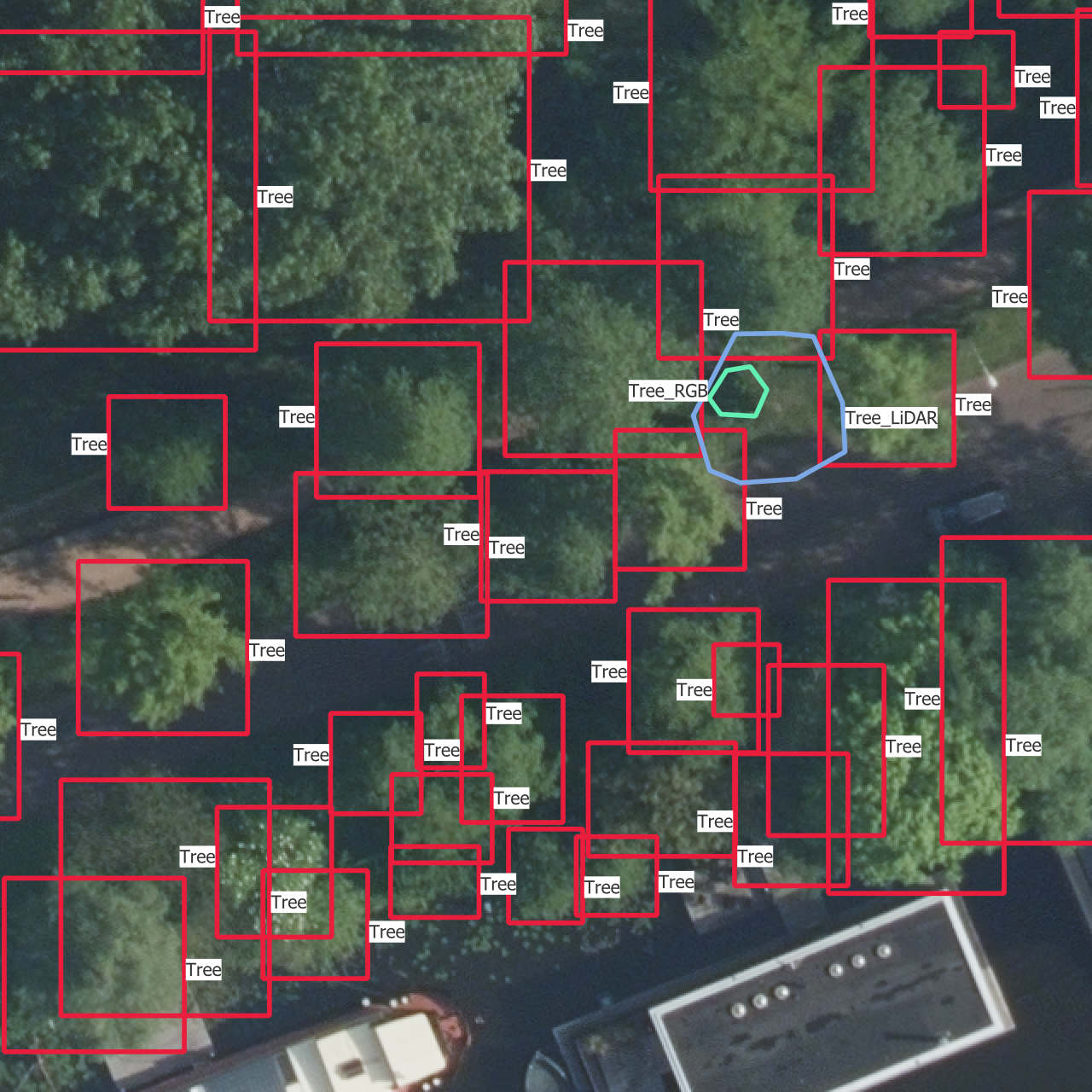
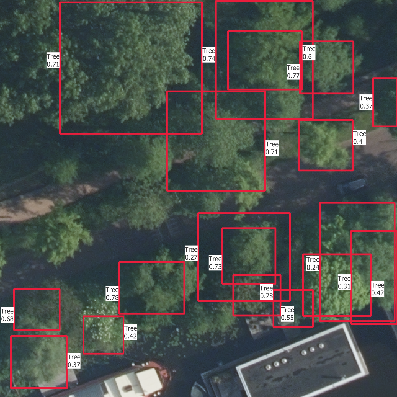
5.3 Covered trees
Then, if we try to look at the performance of the models on the covered trees, which are called “Tree_low_hard” in Figure 5.4, it is also difficult to draw any conclusion. The models have mainly learnt to find trees with the generic “Tree” label, and they are seemingly equally bad at finding the other classes of trees. In Figure 5.4, we can see the performance of two models trained with the same repartition of the data into training, validation and test set. Both models were not agnostic, which means that they learnt to detect each class of trees and label them properly. The one of the left uses the largest number of CHM layers (with Borders = [1, 2, 3, 5, 7, 10, 15, 20] and Disjoint = False), whereas the one on the right only uses the default CHM layer (Borders = []).
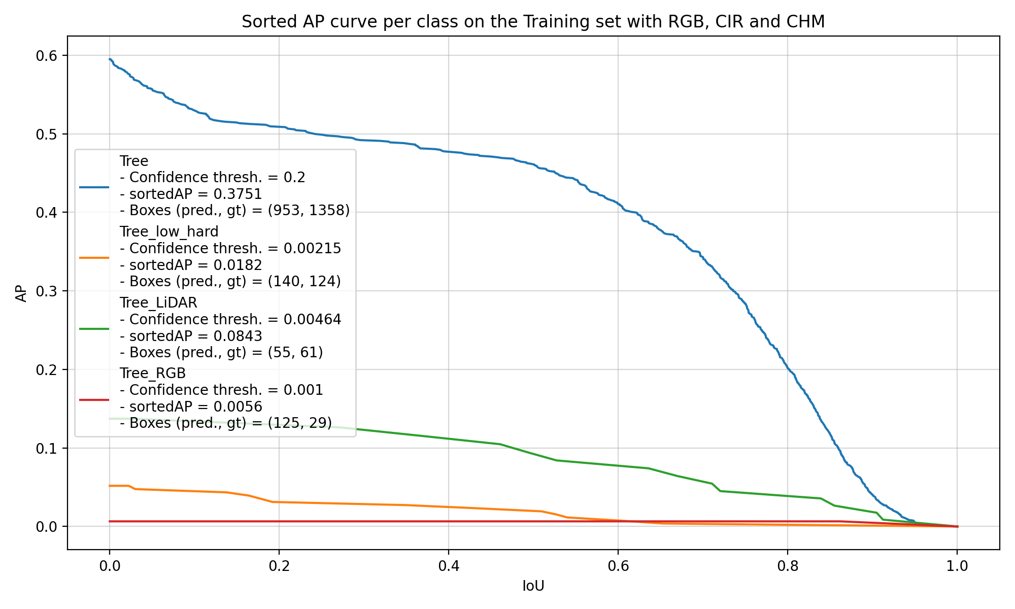
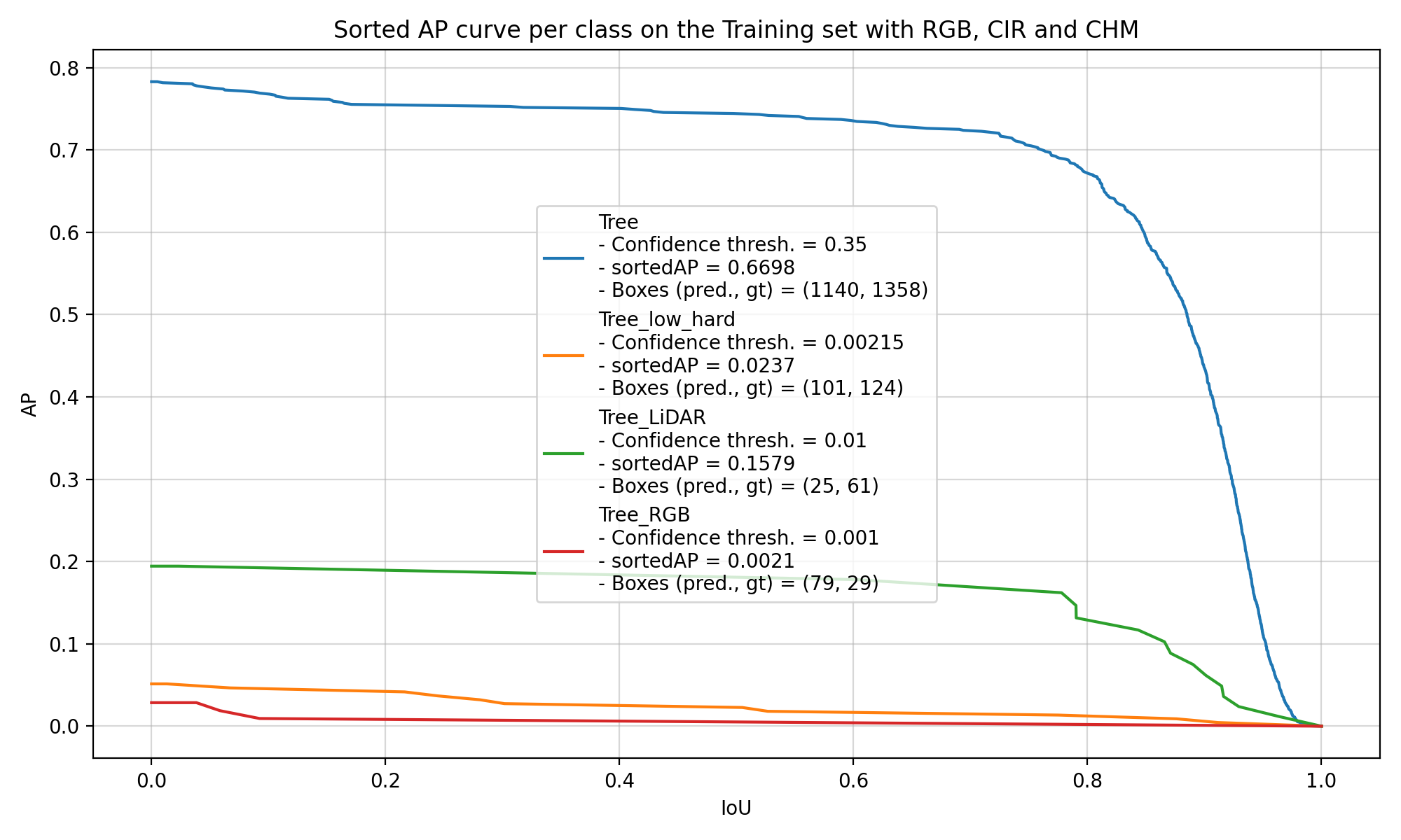
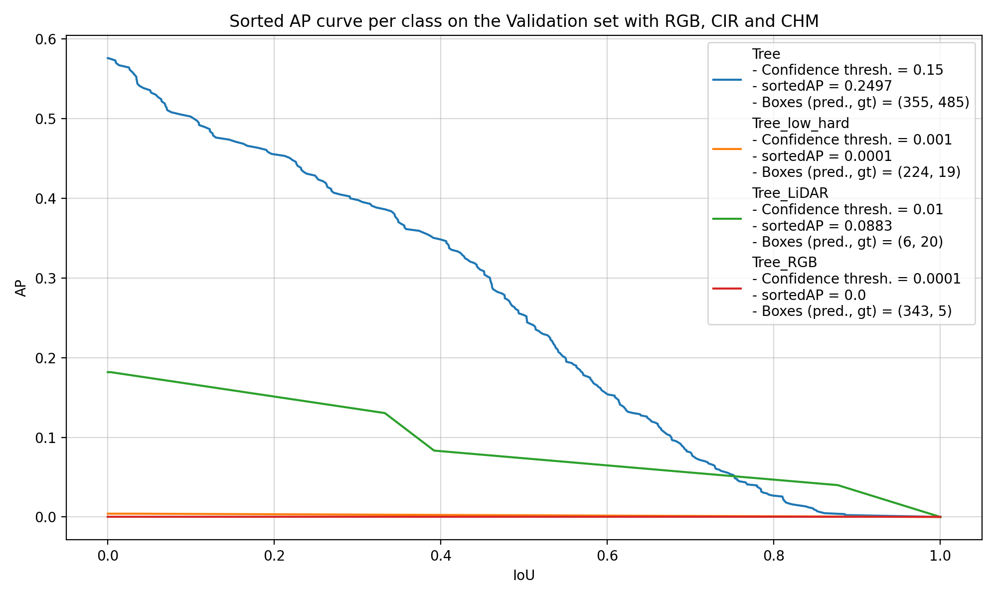
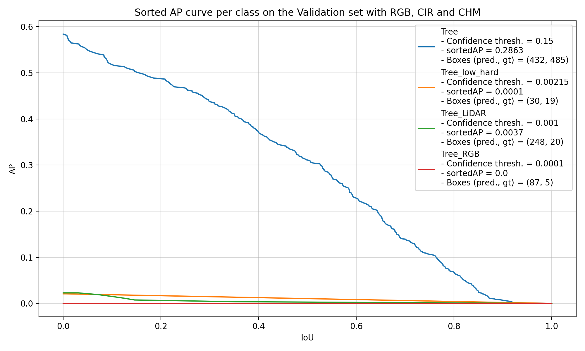
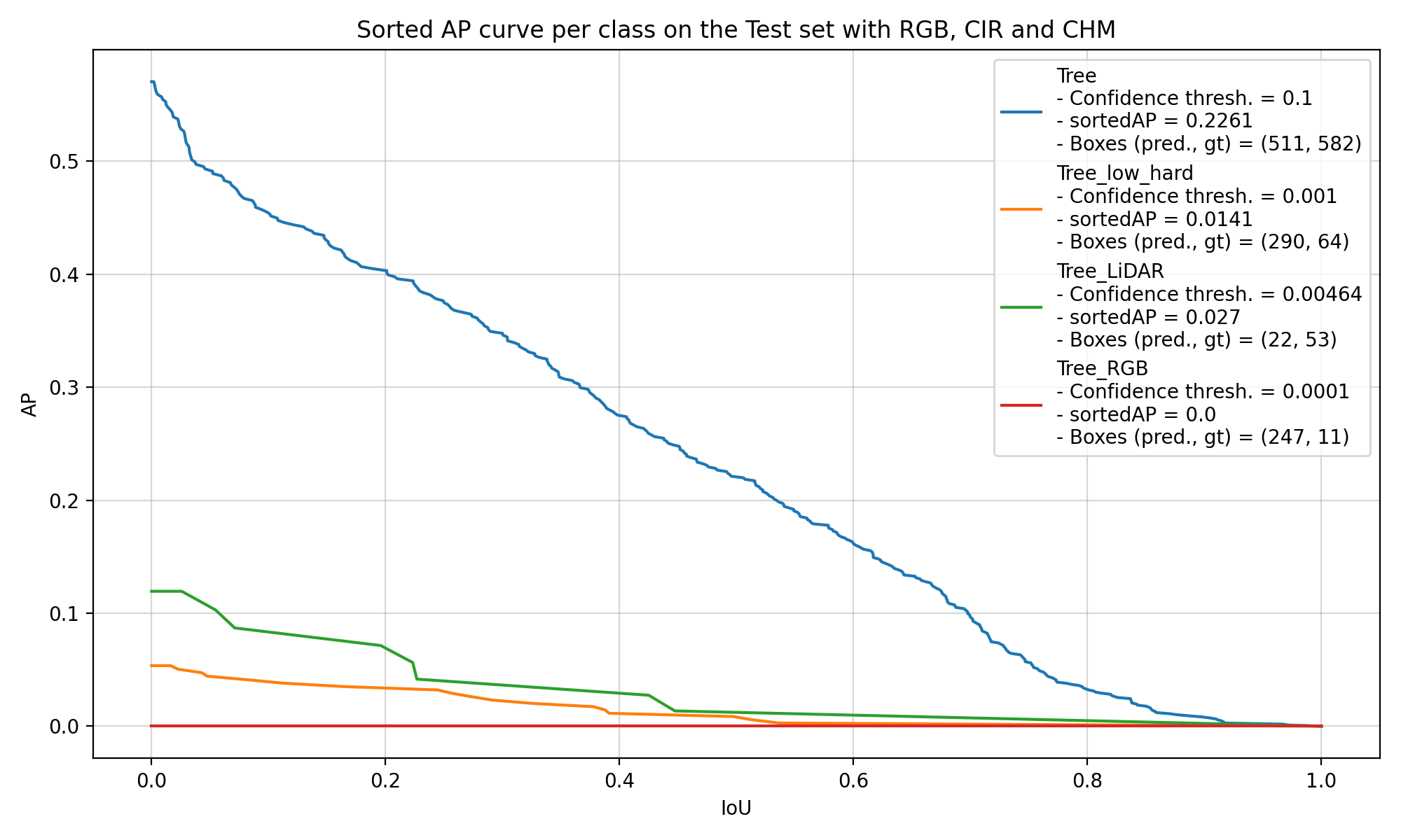
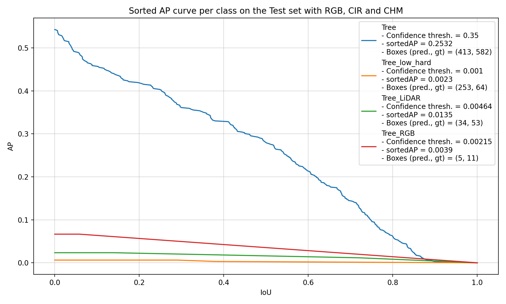
These two examples are really representative of the results of the other models that were trained. There are only 207 covered trees in the dataset, which is too small to get the models to learn to identify them and get solid results when comparing different configurations of CHM layers. Most of the differences that we see come from the normal random variation during the training.
5.4 Visual results
In Figure 5.5 are the outputs of trained models on one instance from each of the training, validation and test sets. The models used are those which results are shown in Figure 5.4.
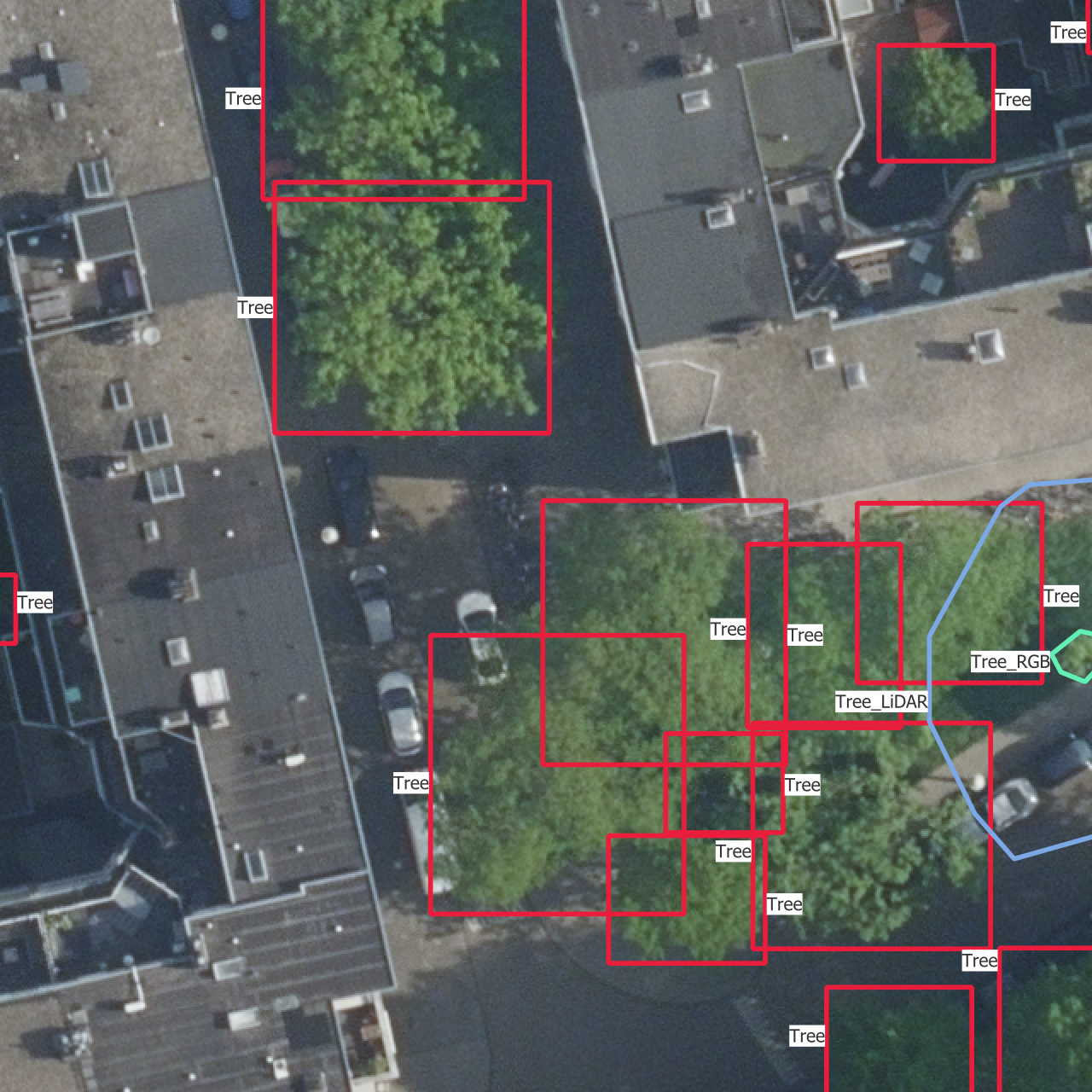
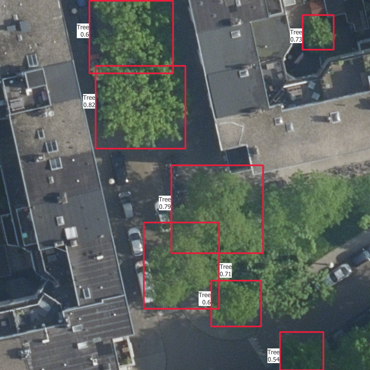
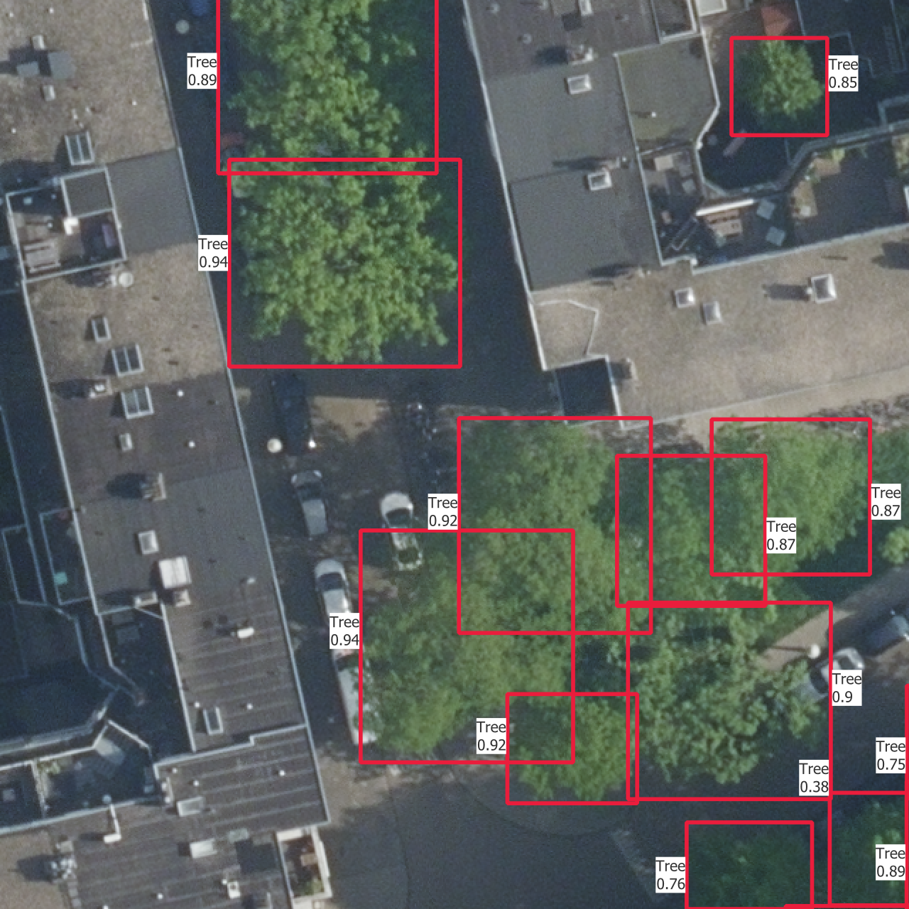
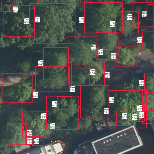
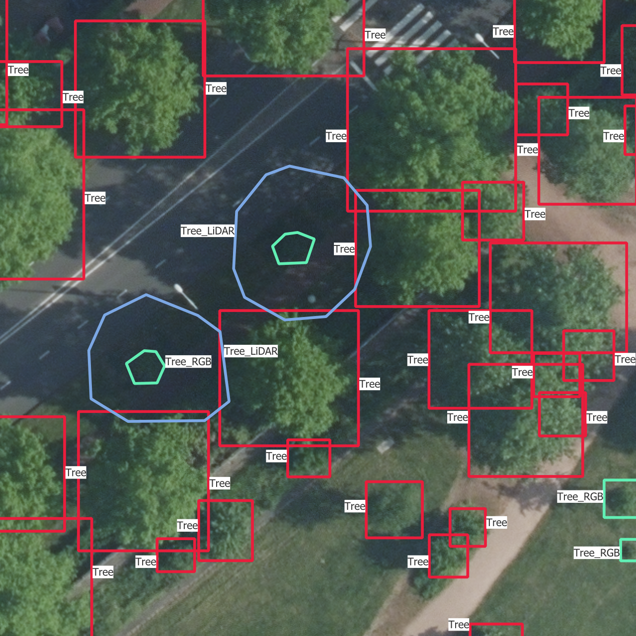
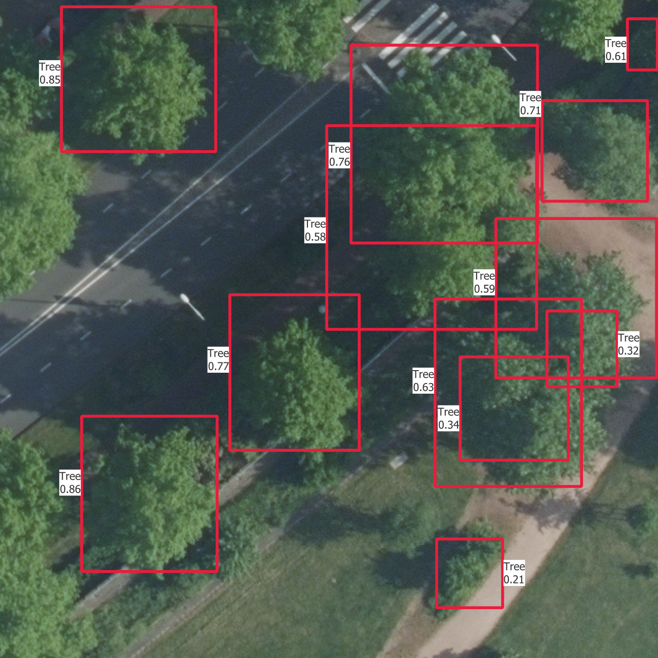
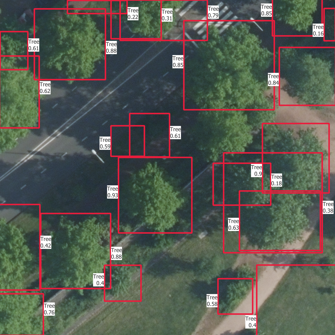
The confidence thresholds used to remove low confidence predictions are the ones that gave the best sortedAP values in Figure 5.4. One aspect that is partly visible here is that all the categories except the basic “Tree” have confidence scores which are so low that they are rejected after the selection with the confidence threshold. This is the reason why there is no predicted bounding box from another class than “Tree”, even though the models do predict boxes with other labels. This is the case on the whole dataset, including the training set, and shows how the models learns more slowly to find the other categories.