4 Model and training
The deep learning model that is used is based on AMF GD YOLOv8, the model proposed in this paper (Zhong et al. 2024).
4.1 Model architecture
The general architecture of the model is conceptually simple. The model takes two inputs in the form of two rasters with the same height and width. The two inputs are processed using the backbone of the YOLOv8 model (Redmon et al. 2016) to extract features at different scales. Then Attention Multi-level Fusion (AMF) layers are used to fuse the features of the two inputs at each scale level. Then, a Gather-and-Distribute (GD) mechanism is used to propagate information between the different scales. This mechanism fuses the features from all scales before redistributing them to the features, two times in a row. Finally, the features of the three smallest scales are fed into detection layers responsible for extracting bounding boxes and assigning confidence scores and class probabilities to them.
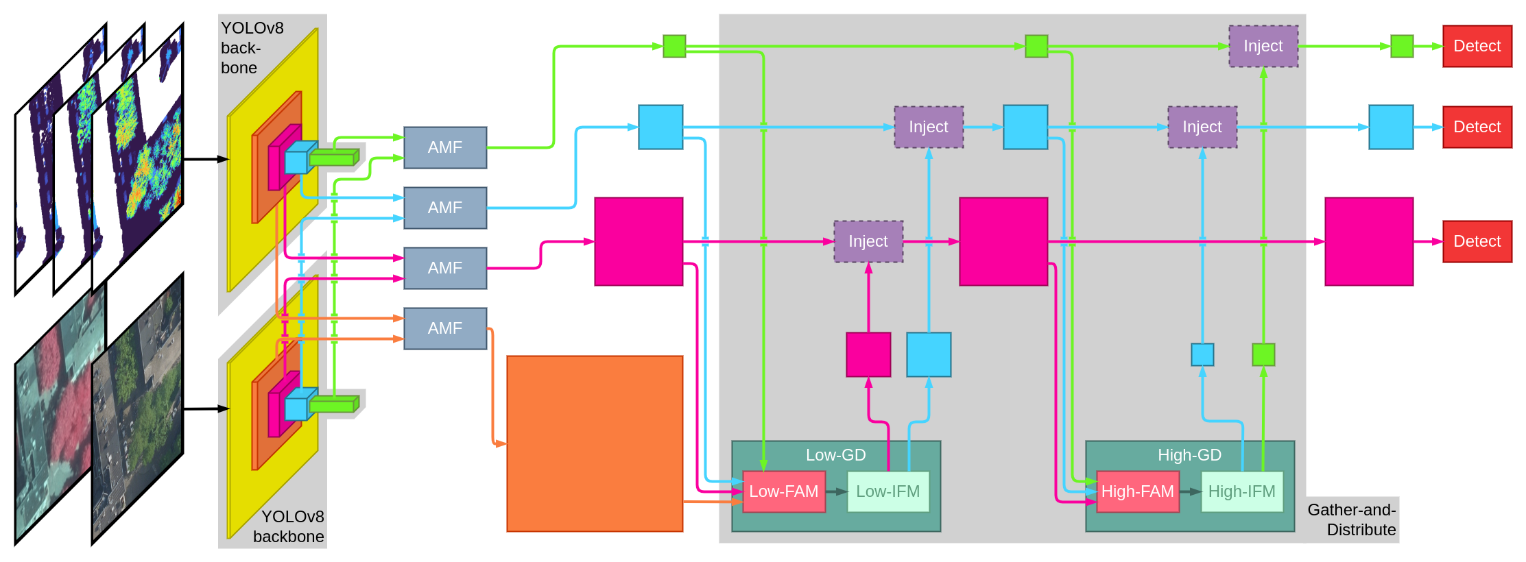
In practical terms, the input rasters have a shape of \(640 \times 640 \times c_{\text{RGB}}\) and \(640 \times 640 \times c_{\text{CHM}}\), where \(c_{\text{RGB}}\) is equal to 6 when using RGB and CIR images, and 3 when using only one of them, and \(c_{\text{CHM}}\) is the number of CHM layers used for the model. Since the resolution that is used is 0.08 m, this means that each image spans over 51.2 m.
The only real modification that I made to the architecture compared to the initial paper is adding any number of channels in the CHM input, while there was only one originally (\(c_{\text{CHM}} = 1\)). Using CIR images in addition to RGB images is also new, but this is a less important modification.
4.2 Training pipeline
The training pipeline consists of three steps. First, the data is pre-processed to create the inputs to feed into the model. Then, the training loop runs until the end condition is reached. Finally, the final model is evaluated on all the datasets.
4.2.1 Data preprocessing
Data pre-processing is quite straightforward. The first step is to divide the dataset into a grid of \(640 \times 640\) tiles. Then, all these tiles are placed into one of the training, validation and test sets.
As for RGB and CIR images, preprocessing only contains two steps: tiling the large images into small \(640 \times 640\) images, and normalizing all images along each channel. When both data sources are used, RGB and CIR images are also merged into images with 6 channels, which will be the input of the model.
As for CHM layers, there are more steps. The first step is to compute a sort of flattened point cloud, by computing the DTM, which represents the height of the ground, and removing this height to the point cloud. Then, for each CHM layer, if the height interval is \([z_\text{bot}, z_\text{top}]\), all the points which have a height \(h\) such that \(z_\text{bot} \leq h \leq z_\text{top}\) are extracted, and the DSM is computed for this smaller point cloud. Since the ground height was already removed from the point cloud, this DSM is the CHM. Then, all the layers are merged into one raster with multiple channels and the whole raster is normalized with the average and the standard deviation over all channels. Finally, these rasters are tiled exactly like RGB and CIR images, which gives the inputs of the model.
All these operations are conceptually simple, but they can be computationally expensive. Therefore, I put effort into accelerating with different methods. First, I made sure to save the most important and generic elements to avoid useless computations every time the model is trained again, without saturating the memory. Then, I also implemented multi-threading for every possible step to improve the raw speed of preprocessing. Finally, performance is also the reason why normalization if performed during preprocessing instead of during the initialization of the data in the training loop.
4.2.2 Training loop
The training loop is very generic, so I will only mention the most interesting parts. First, an Adam optimizer and a basic learning rate scheduler with a multiplier at each epoch i which is \(1/\sqrt{i+2}\) are used.
Then, since the batch size cannot be very large because of the GPU memory space required by all the images, there is the possibility to perform gradient accumulation, which means that backward propagation won’t be performed with each batch, but instead every two or more batches. The idea behind this is to add more stability to the training, since back-propagating on only a few images is prone to overfitting on a set of examples which are not representative of the whole dataset.
As for the criterion to stop the training session, the loss on the validation set is used. Once this loss hasn’t improved for 50 iterations over the whole dataset, the training stops and the model that had the best validation loss is saved.
Besides these details, the training loop is very generic. We loop over the entire training set with batches to compute the loss and perform gradient back-propagation. Then the loss is computed over the validation set and stored as the metric that decides when to stop.
4.2.3 Output postprocessing
Regarding postprocessing of the output of the model, there a few things to mention. First, the model outputs a lot of bounding boxes, which have to be cleaned using two criteria. The first criterion is the confidence score, which is used by setting a threshold below which bounding boxes are discarded. The second criterion is the intersection over union (IoU) with other bounding boxes. IoU is a metrics used to quantify how similar two bounding boxes are. It is a value between 0 and 1, which formula is:
\[ \text{IoU}(A, B) = \frac{\text{area}(A \cap B)}{\text{area}(A \cup B)} \]
This metrics can be used to detect bounding boxes which are too similar to each other. This allows to simply keep the bounding box with the highest confidence score when two bounding boxes have an IoU larger than a certain threshold. This process based on IoU to eliminate duplicate bounding boxes is called non-maximum suppression.
For the evaluation, the process is a little different, because non-maximum suppression is performed but the confidence threshold used to filter predicted boxes is 0. The main metric that is computed is called sortedAP (Chen et al. 2023), which is an evolution of the mean (point) average precision (mAP). mAP is defined as follows:
\[ \begin{array}{rcl} \text{mAP} & = & \frac{1}{N} \sum\limits_{t\in T} \text{AP}_t \\ \text{AP}_t & = & \frac{{TP}_t}{{TP}_t + {FP}_t + {FN}_t} \end{array} \]
where \(T=\{t_1, t_2, \dots, t_N\}\) is a list of IoU threshold values, \({TP}_t\) are the true positives when the the IoU threshold is \(t\), \({FP}_t\) are false positives and \({FN}_t\) are false negatives. The reason why \(TP\), \(FP\) and \(FN\) depend on \(t\) is that a bounding box is considered to be true if its IoU with one of the ground-truth bounding boxes is larger than \(t\).
sortedAP is an improvement over this method because there is no need to select a list of IoU threshold values. Predicted bounding boxes are sorted according to their confidence score which allows to compute AP incrementally for any value of \(t\). Then, the area of the curve of the AP with respect to the IoU threshold is used as a metric, between 0 and 1, 1 being the best possible value. You can see in Figure 4.1 an example of the output of the sortedAP method. The curves represent the AP at any IoU threshold value. Then, the integral of this curve gives the value of sortedAP, which is displayed in the legend here.

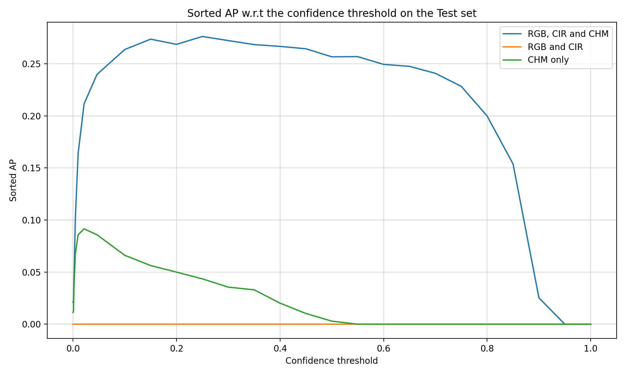
Finally, it is necessary to choose a fixed confidence threshold to compute the curve, because this value decides which boxes will be kept and how the predicted and ground-truth boxes will be matched. Therefore, the value of the best confidence threshold has a very high impact over the value of sortedAP, and cannot easily be determined during the training, as the confidence of the model evolves quickly. Therefore, computing sortedAP for different confidence threshold allows to always estimate the best performance it can have. Figure 4.2 shows how the value of sortedAP evolves and how the confidence threshold values in the previous figure (Figure 4.1) were chosen.